

Microsoft Excel offers two different methods to help you compare two lists and highlight missing items in each. You can choose to highlight missing items in both lists or in just one. We'll show you how.
See also: How to divide numbers in Microsoft Excel

The Quick Way: Highlight Unique Cells for List Comparison
A quick way to compare two lists in spreadsheet is to use Excel's unique highlighting feature. This feature highlights items in one list that aren't in the other list. This way, you know exactly which items are missing from your lists.
See also: How to import data from a PDF into Microsoft Excel
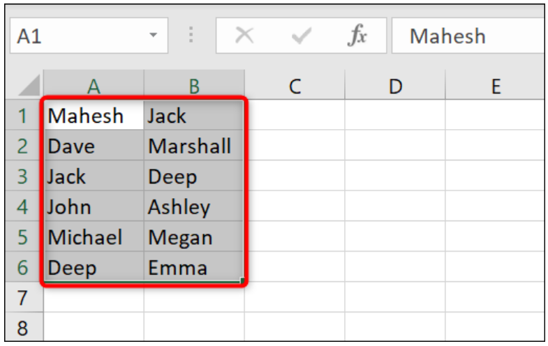
To use the method, first select the lists you want to compare in your spreadsheet.
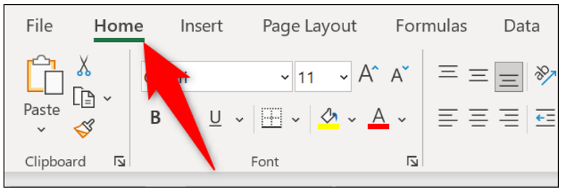
While your lists are highlighted, on the Excel ribbon at the top, click the “Home” tab.
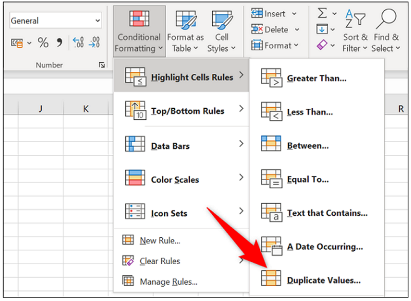
On the Home tab, in the Styles group, click Conditional Formatting > Highlight Cells Rules > Duplicate Values.
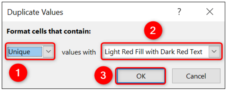
In the “Duplicate Values” box, click “Duplicate” and select “Unique.” Click the second drop-down menu and choose how you want to highlight missing items. To specify your own formatting, select “Custom Format” from the menu.
See also: Microsoft Excel: How to create a data entry form
Then, apply your changes to your lists by clicking “OK”.
Excel will highlight the missing items in your lists. For example, in your first list, you will have highlighted those items that are missing from the second list, and so on.
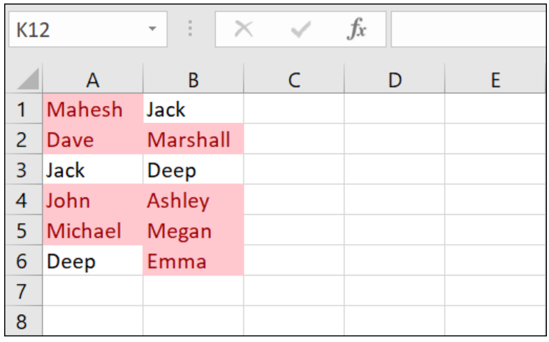
And you are ready!
The formula way: Use conditional formatting to compare lists
The above method highlights items in both of your lists. If you want to highlight only items that are missing in a specific list, use a formula with conditional formatting as explained below.
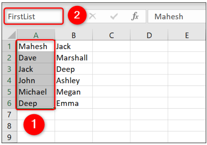
First, in your spreadsheet, select all the rows of your first list. Then, in the upper-left corner, click the text box, type FirstList, and press Enter. This assigns a unique name to your range of cells, which allows you to reference all of those cells using a single name.
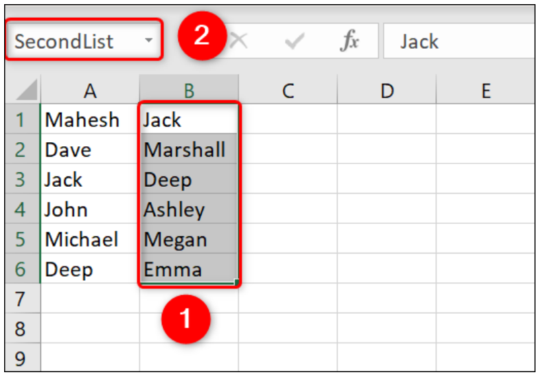
Give your second list a unique name by first selecting all the rows in your list. Then, in the upper-left corner, click the text box, type SecondList, and press Enter.
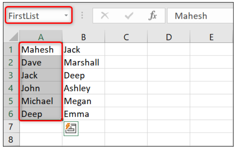
Select all the rows of your first list by clicking the text box in the upper left corner and selecting “FirstList.”
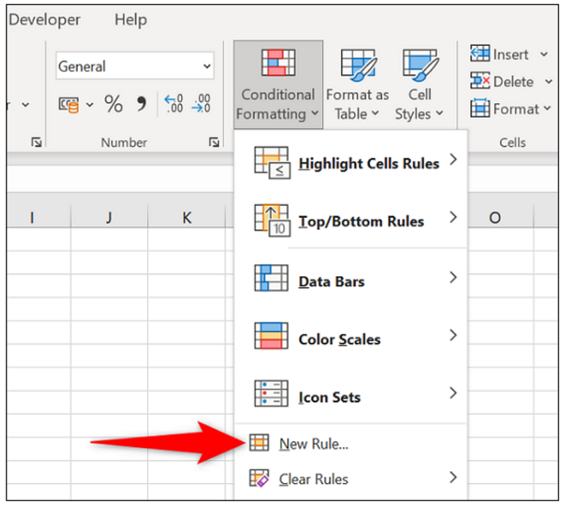
On the Excel ribbon at the top, click the “Home” tab and select Conditional Formatting > New Rule.
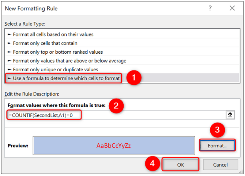
In the “New Formatting Rule” window, you will specify how missing data will be highlighted. In this window, under “Select a Rule Type,” select “Use a Formula to Determine Which Cells to Format.”
In the “Format Values Where This Formula is True” box, type the following:

Select the “Format” button and specify how you want to format the missing items in your list. Then save your changes by clicking “OK.”.
Back in the spreadsheet, Excel has highlighted the items in the first list that are missing from the second list. And you're done!
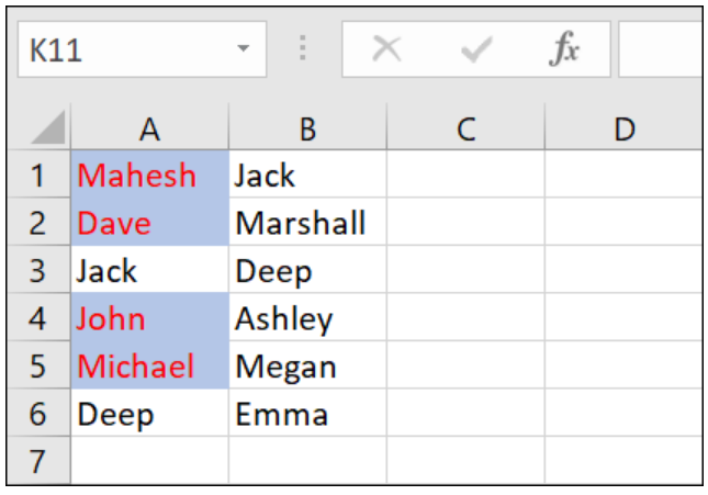
And this way you quickly perform a comparison of two different lists in Excel spreadsheets.
Information source: howtogeek.com
